 |
LandscapeDNDC 1.37.0
|
|
LandscapeDNDC 1.37.0
|
The shape of tree stems is defined by the relation between tree height, diameter and stem volume. While the volume is only constraint by stem biomass and wood density, a change in volume can thus be related to a change in tree height and diameter based on:
Because the taper function is based on tree height and diameter at breast height - but the latter is unavailable for trees shorter than 1.3 m - it is assumed that the form of short trees \((height < 0.5 \cdot HLIMIT)\) is that of a cone. Thus, dimensional growth can be determined from volume growth with only a given height-diameter ratio. The stem volume of large trees \((height > HLIMIT)\) is determined by a taper function.
Both calculations of stem dimensional developments (for short as well as tall trees) require an indication of the optimal height-diameter relationship, which is given as:
\[ hd\_{opt} = (HDMIN + (HDMAX - HDMIN) \cdot exp(-HDEXP \cdot dbh)) \cdot competition\_{factor} \]
with
If the optimum height:diameter ratio (hd ratio) can be achieved based on the current tree dimensions, it is realized. Otherwise diameter growth will be established iteratively with a hd ratio as close as possible to the optimum one until the new wood volume (vol, m3) matches the calculated volume growth (see taper).
The competition factor is calculated empirically as:
\[ competition\_{factor} = (\frac {areacover\_{openrange} }{DFLIMIT} ) ^ {DFEXP} \]
To estimate the stand density impact on crown size, crown coverage without competition is calculated first:
\[ areacover\_{openrange} = (dbh \cdot cdr\_{open})^2 \cdot PI \cdot 0.25 \cdot N\_{trees} \]
\[ cdr\_{open} = CDR_P1 + CDR_P2 \cdot log(dbh) + CDR_P3 \cdot log(height) \]
with
For short trees, a cone-shaped trunk is assumed where the relationship between volume, height, and (base) diameter can be calculated as:
\[ vol_{cone} = \frac {PI \cdot (d\_{base} \cdot 0.5) ^ {2} \cdot height} {3.0} \]
All dimensional changes based on wood volume increase can thus be derived
considering the previously defined height-diameter relationship \( f_{hd}(d) \):
\[ height = \frac {vol_{cone} \cdot 3.0} {PI \cdot (d\_{base} \cdot 0.5) ^ {2} } \]
\[ d\_{base} = \frac {height} { hd\_{opt} } \]
with
The taper function that has been selected for the calculation of stem volume [ \(m^3\)] depends on tree height \( h [m] \) and tree diameter \( d [m] \):
\[ vol_{tap} = 0.001 \cdot (100 \cdot dbh)^{TAP\_{P1} } \cdot height^{TAP\_{P2}} \cdot exp(TAP\_{P3}) \]
with
The taper parameters \( TAP_P1, TAP_P2, TAP_P3 \) are species-specific. Default parameters for coniferous trees are:
Default parameters for deciduous trees are:
According to the taper equation, tree height is can be defined in dependence on tree volume \( V \) [m \(^3\)] and tree diameter at breast height [m]:
\[ height = \left( \frac{vol_{tap}}{0.001 \cdot (100 \cdot dbh)^{TAP_P1}} \cdot exp(TAP_P3) \right)^{\frac{1}{TAP_P2}} \]
Also, tree diameter at breast height can be calculated with this equation based on tree volume \( V \) [m \(^3\)] and tree height [m] using the same taper parameters:
\[ dbh = 0.01 \cdot \left( \frac{vol_{tap}}{0.001 \cdot height^{TAP_P2}} \cdot exp(TAP_P3) \right)^{\frac{1}{TAP_P1}} \]
For larger trees ( \( h > HLIMIT \)), diameter at ground height is determined depending on diameter at breast height \( dbh \) and tree height \( height \):
\( d_{base} = dbh + \frac{HLIMIT}{height} \cdot dbh \)
For \( \; 0.5 \cdot HLIMIT < height \le HLIMIT \; \) a linear transition between the two shapes is assumed:
\[ vol = \phi \; vol_{tap} + (1.0 - \phi) \; vol_{cone} \]
with \( \phi \) representing a linear scaling factor. Accordingly, the diameter used for allometric scaling (e.g. regarding height/diameter ratio) is shifting during this period between ground height (dbase) and breast height (dbh), and is regarded as effective tree diameter ([15]). As described for the volume, the effective tree diameter is defined by a linear transition using the scaling factor \( \phi \)):
\[ d_{eff} = (1 - \phi) \; d_{base} + \phi \; dbh \]
Since the optimum height-diameter ratio might not be achievable given the dimensions of the previous state, a change in trunk volume is translated into height and diameter changes iteratively:
\begin{eqnarray*} d_{test} = DBHLIMIT \\ \text{while} \; (vol_{test} < vol): \\ height_{test} &=& d_{test} \cdot hd\_{opt}(d_{test}) \\ vol_{test} &=& V(d_{test}, height_{test}) \\ d_{test} &=& d_{test} + increment \end{eqnarray*}
With the increment used for diameter modification is plus or minus 10, 1, and 0.5 cm steps.
Stem volume for small trees is approached with a cone function iteratively approachng a new volume with a fixed HD ratio With the increment used for diameter modification is plus or minus 1 mm steps.
Since the optimum height-diameter ratio might not be achievable given the dimensions of the previous state, a change in trunk volume is translated into height and diameter changes iteratively:
\begin{eqnarray*} d_{test} = DBHLIMIT \\ \text{while} \; (vol_{test} < vol): \\ height_{test} &=& d_{test} \cdot hd\_{opt}(d_{test}) \\ vol_{test} &=& V(d_{test}, height_{test}) \\ d_{test} &=& d_{test} + increment \end{eqnarray*}
With the increment used for diameter modification is plus or minus 10, 1, and 0.1 cm steps.
The crown is generally described by crown length, diameter and a shape function that defines the extension of the crown in each canopy layer. The concept is descript in [28]. The resulting volume is also used to calculate the total demand of branches. Since it is assumed that foliage biomass scales linearly with crown volume, the shape function used to describe the relative canopy volume of each layer and the foliage biomass distribution within the canopy is the same. It is documended under veglibs_biomass_distribution.
The branch fraction is used to calculate the stem biomass and volume that is needed for tree dimensional growth (Dimensional growth). It is EITHER defined using the crown size by assuming a specific branch density per unit volume (Branch fraction from canopy volume) or based on species-specific limit values (Branch fraction from stem diameter). See option settings in Model options.
The crown volume is calculated assuming that every layer can be described as a disc with a horizontal extension defined by the biomass distribution function veglibs_canopy. The total volume can then be integrated across all canopy layers.
\[ f\_{branch} = \frac {m\_{branch} } { (m\_{stem} + m\_{branch}) } \]
\[ m\_{branch} = DBRANCH \cdot can\_{vol} \]
\[ can\_{vol} = \int ( ( \frac {fFol_{fl} } {fFol\_{max} } \cdot crown\_{diam} )^{2} \cdot PI \cdot 0.25 \cdot hfl_{fl} ) \]
with:
If this option is selected (Model options), the branch fraction is empirically related to stem diameter at breast height (dbh). Since the development of this term is different in young seedlings (where no dbh is available) and mature trees, branch fraction is calculated as the maximum of two functions:
\[ f\_{branch} = max(fbranch\_{young}, fbranch\_{mature}) \]
For young trees, a maximumum value is intiated that decreases steeply with increasing size, expressed as diameter at ground height.
\[ fbranch\_{young} = FBRAF\_{Y} \cdot ( 1.0 - exp( FSLOPE\_{Y} \cdot dbas) )^{FEXP\_{Y}} \]
After a minimum branch fraction has reached, it is slowly increasing again approaching a final value for mature trees.
\[ fbranch\_{mature} = FBRAF\_{M} + (1.0 - FBRAF\_{M}) \cdot exp(FSLOPE\_{M} \cdot \frac {dbh}{DIAMMAX} ) \]
with
Crown diameter calculation is based on the open-range calculations that depend on breast-height diameter and tree height as presented by Condes and Sterba [15].
\[ crown\_{diam} = CDR\_{P1} + (CDR\_{P2} \cdot log(dbh)) + (CDR\_{P3} \cdot log(height)) \]
with
In case that the canopy coverage of crowns calculated for open-grown trees is larger that a predefined species-specific threshold value (MORDCROWD), the crown diameter is reduced by a reduction factor that restricts the coverage to the threshold.
For all vegetation types other than woody species, crown length is equal to height. For trees, it is calculated depending on the setup-option selected (options depicted in 'PSIM' descriptions).
The first option is to calculate crown length based on an allometric relationship to tree height and diameter at breast height (= option height):
\[ crown\_{length} = min(HLIMIT, height\_{eff} \cdot CB ) \]
\[ height\_{eff} = height - HREF \cdot (1.0 - \frac {dbh}{DIAMMAX} ) \]
with: \( \text{h}_{\text{cs}} \): height at canopy start
\( \text{h}_{\text{max}} \): height at canopy top
\( DIAMMAX \): tree diameter at which a mature state is defined
\( CB \): relation between crown base height and top height at a mature state (dbh >= DIAMMAX)
\( HREF \): tree height at which crown base height starts to increase
The second option is to calculate crown length from crown diameter (option 'diameter') according to [66] .
\[ crown\_{length} = CL\_{P1} \cdot ( crown\_{diam} ) ^ {CL\_{P2} } \]
with:
Crown length is limited by tree height. The crown base height (or crown start) is defined as tree height - crown length.
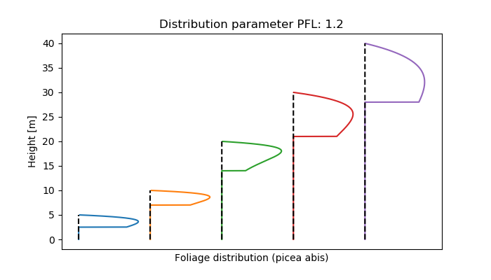
The distribution of foliage biomass \( m(z) \) within the canopy depends on canopy length with a tendency to put more weight to the bottom of the distribution with larger length ([31], [32]):
\[ m(z) = M \cdot \frac{r_{ih} f(z)}{\int r_{ih} f(z)} \\ r_{ih} = \frac{CL - z}{CL} \\ f(z) = p^{100 \frac{z}{CL^2}} \]
\( CL \): canopy length (difference between start and end of canopy, m)
\( z \): distribution depth for which the percentage foliage should be defined (between 0-1, refers to canopy start and top height)
\( p \): shape parameter
If no other options are defined, new root biomass is distributed to the different soil layers according to the selected root distribution scheme (standard, sigmoidal, or exponential). Therefore, the overall distribution stays constant.
Root biomass distribution may be limited by various environmental (soil, climate) restrictions. These restrictions are calculated separately for all relevant layers, following [3]. A value of 0 corresponds to full restriction (no growth), a value of 1 stands for optimum conditions. The actual root mass distribution is based on an optimum root biomass distribution assuming either exponential or sigmoidal functions, which is then modulated by the restrictions in every soil layer. The downwards growth rate (GZRTZ) is defined as an optimum value, and is adjusted by the restrictions present in the soil of the root front. There is no active redistribution of old root biomass but root biomass which is not supported by growth will continously decrease due to senescence.
Before germination period, carbon distribution is done empirically. Afterwards, the restrictions are caluclated as follows:
The combination of individual restrictions is then done following [3] :
\[ \Delta rd_{red} = \Delta rd_{pot} \cdot \min\left(STP, \min(SST,SAI,SCF)^{0.5} \right), \]
The restrictions in the bottom layer are assumed to represent a reasonable simplification as long as the time steps are small so that root elongation is also small in comparison to the soil layer widths.
This functions determines the target depth of the roots under optimum conditions in this time step. A linear increase with the slope GZRTZ is assumed.
\[ S_{Fc}(sl) = 1 - stone\_content [\text{volume fraction}](sl) \]
\[ S_{BD} = 1, \quad BD < BD_O\,,\\ S_{BD} = \frac{BD_X-BD}{BD_X-BD_O}, \quad BD_O \leq BD \leq BD_X\,,\\ S_{BD} = 0, \quad BD > BD_X\, , \]
where the threshold \(BD_O\) is the bulk density at which root growth is first affected, and \(BD_X\) is the bulk density above which no root growth occurs. Following [3], these parameters can be estimated from the sand content [weight fraction] \(sand\)\[ BD_O = 1.1 + 0.005 \cdot sand\, ,\\ BD_X = 1.6 + 0.004 \cdot sand\, . \]
\[ S_{AI} = S_{FT} + (1- WFP) \cdot \frac{1- S_{FT}}{1 - CWP}, \quad WFP \geq CWP \,,\\ S_{AI} = 1, \quad WFP < CWP \,. \]
With the fraction of water filled pore space calculated as:\[ WFP = \frac{\text{water filled porosity}}{\text{total porosity}} \]
The critical value of water filled pore space depends on the clay content:\[ CWP = 0.4 + 0.004 \cdot clay \, . \]
IV) Restriction due to temperature stress If the soil temperature is below a critical value ($T_{BS}$), root growth doesn't occur. Similar, too hot conditions also restricted carbon allocation into roots. Here, it is assumed that the limitations occur symmetrically around an species-specifc optimum temperature $T_{OP}$, using a sinus function around an optimum temperature to describe the dependency.
\[ S_{TP} = 0, \quad T<T_{BS} \,,\\ S_{TP} = \sin\left( \frac{\pi}{2} \frac{T-T_{BS}}{T_{OP}-T_{BS}}\right), \quad T_{BS} \leq T \leq 2T_{OP} - T_{BS}\,,\\ S_{TP} = 0, \quad T > 2T_{OP} - T_{BS}\,. \]

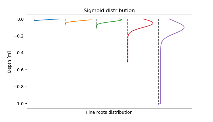
The root mass distribution decreases sigmoidel with the soil depth:
\[ m(z) = M \cdot \frac{f(z)}{\int f(z)} \\ f(z) = \left( \frac{e^{(-\frac{(z - 0.1 \cdot RD)^2}{0.01 \cdot RD}}}{RD} + 0.1 \cdot L \right) \]
with \( M \): root growth (kg m-2)
\( RD \): root depth (m)
\( z \): distribution depth for which the percentage roots should be defined (between 0-1, from upper soil boundary to rooting depth)
In absolute values of the soil layer, s [cm], for all rooted layers, the distribution is defined as
\[ f(z) = \left( \frac{e^{(-\frac{s - 10}{120}}}{10} + 0.005 \right) \cdot \Delta s \]
with the layer width delta s. Note, that if the function is called from Plamox, instead of the value 120 for rootwidth, a value of 200 is used.
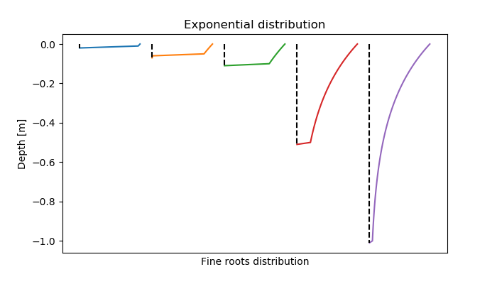
The root distribution decreases exponentially with the soil depth:
\[ m(z) = M \cdot \frac{f(z)}{\int f(z)} \\ f(z) = \exp(-EXP\_ROOT\_DISTRIBUTION \cdot z) \]
with: \( M \): root growth (kg m-2)
\( z \): distribution depth for which the percentage roots should be defined (between 0-1, from upper soil boundary to rooting depth)
\( EXP\_ROOT\_DISTRIBUTION \): species-specific distribution parameter
While root biomass is defined by one of the rooting distribution schemes, root length is calculated based on root biomass but considering a specific root length for every single soil layer. Specific root lenghts scales linearly between \(SRLMIN\) and \(SRLMAX\) as:
\[ specific\_{rootlength}_{sl} = SRLMAX - dvsFlush \cdot (SRLMAX - SRLMIN) \cdot scale_{sl}; \]
\[ scale = 1.0 - \frac {depth_{sl}} {depth\_{root}} \]
with
Specific root length calculated for every rooted layer
Nitrogen uptake depends on temperature
Nitrogen uptake includes:
Assumptions:
Ratio between sapwood and foliage area (Huber Value) The sapwood to foliage area relationship (m2 sapwood area m-2 leaf area) is calculated following [44], which is assumed to scale linearly with tree height.
\[ qsfa = QSF\_{P1} + height \cdot QSF\_{P2} \]
with
Vernalization after [34].
Influence of vernalization starts as soon as accumulated growing degree days \( AGDD \) are greater than half of the required growing degree days for the state of flowering \( GDD\_FLOWERING \):
\[AGDD > 0.5 \cdot GDD\_FLOWERING \]
Chill factor \( f_{chill} \) is given by:
\[ f_{chill} = 1 - \frac{AGDD - 0.5 \cdot GDD\_FLOWERING}{0.5 \cdot GDD\_FLOWERING} + \frac{ACU}{CHILL\_UNITS} \]
wherein \( ACU \) and \( CHILL\_UNITS \) refer to accumulated chill units and required chill units for complete vernalization, respectively. The factor \( f_{chill} \) is bound between 0 and 1.
Accumulated chilling units \( ACU \) are given by:
\begin{eqnarray*} ACU &=& \sum CU \\ CU &=& \frac{CHILL\_TEMP\_MAX - T_{avg}}{CHILL\_TEMP\_MAX} \end{eqnarray*}
\( CHILL\_TEMP\_MAX \) and \( T_{avg} \) refer to a species-specific parameter and daily mean temperature, respectively.
Exponential drought stress factor \( \phi_d \):
\[\phi_d = \frac{1 - e^{-f_{H2O} gsslope}}{1 - e^{-gsslope}} \]
Related literature: Soil drought impact on stomatal conductance [69]
\[\phi_d = 1.016 - 0.016 \cdot e^{ 4.1 \cdot ( 1.0 - _fh2o)} \]
A general relationship for 5 tree species was developed by [26]
\[\phi_d = (1.154 + 3.0195 \cdot _fh2o - ((1.154 + 3.0195 * _fh2o)^2 - 2.8 \cdot 1.154 \cdot 3.0195 \cdot _fh2o)^{0.5}) /1.4)); \]
Linearly calculated soil drought impact on stomatal conductance ( \( \phi_d \)) according to [72] (more flexible due to species-specific sensitivity):
\[\phi_d = min \left ( \frac{f_{H2O}}{f_{H2O,ref}} , 1 \right ) \]
Non-stomatal impact of drought stress [67].